The goal of a just-in-time compiler for a dynamic language is obviously to
improve the speed of the language over an implementation of the language that
uses interpretation. The first goal of a JIT is thus to remove the
interpretation overhead, i.e. the overhead of bytecode (or AST) dispatch and the
overhead of the interpreter's data structures, such as operand stack etc. The
second important problem that any JIT for a dynamic language needs to solve is
how to deal with the overhead of boxing of primitive types and of type
dispatching. Those are problems that are usually not present in statically typed
languages.
Boxing of primitive types means that dynamic languages need to be able to handle
all objects, even integers, floats, etc. in the same way as user-defined
instances. Thus those primitive types are usually boxed, i.e. a small
heap-structure is allocated for them, that contains the actual value.
Type dispatching is the process of finding the concrete implementation that is
applicable to the objects at hand when doing a generic operation at hand. An
example would be the addition of two objects: The addition needs to check what
the concrete objects are that should be added are, and choose the implementation
that is fitting for them.
Last year, we wrote a blog post and a paper about how PyPy's meta-JIT
approach works. These explain how the meta-tracing JIT can remove the overhead
of bytecode dispatch. In this post (and probably a followup) we want to explain
how the traces that are produced by our meta-tracing JIT are then optimized to
also remove some of the overhead more closely associated to dynamic languages,
such as boxing overhead and type dispatching. The most important technique to
achieve this is a form of escape analysis that we call virtual objects.
This is best explained via an example.
Running Example
For the purpose of this blog post, we are going to use a very simple object
model, that just supports an integer and a float type. The objects support only
two operations, add, which adds two objects (promoting ints to floats in a
mixed addition) and is_positive, which returns whether the number is greater
than zero. The implementation of add uses classical Smalltalk-like
double-dispatching. These classes could be part of the implementation of a very
simple interpreter written in RPython.
class Base(object):
    def add(self, other):
        """ add self to other """
        raise NotImplementedError("abstract base")
    def add__int(self, intother):
        """ add intother to self, where intother is a Python integer """
        raise NotImplementedError("abstract base")
    def add__float(self, floatother):
        """ add floatother to self, where floatother is a Python float """
        raise NotImplementedError("abstract base")
    def is_positive(self):
        """ returns whether self is positive """
        raise NotImplementedError("abstract base")

class BoxedInteger(Base):
    def __init__(self, intval):
        self.intval = intval
    def add(self, other):
        return other.add__int(self.intval)
    def add__int(self, intother):
        return BoxedInteger(intother + self.intval)
    def add__float(self, floatother):
        return BoxedFloat(floatother + float(self.intval))
    def is_positive(self):
        return self.intval > 0

class BoxedFloat(Base):
    def __init__(self, floatval):
        self.floatval = floatval
    def add(self, other):
        return other.add__float(self.floatval)
    def add__int(self, intother):
        return BoxedFloat(float(intother) + self.floatval)
    def add__float(self, floatother):
        return BoxedFloat(floatother + self.floatval)
    def is_positive(self):
        return self.floatval > 0.0
Using these classes to implement arithmetic shows the basic problem that a
dynamic language implementation has. All the numbers are instances of either
BoxedInteger or BoxedFloat, thus they consume space on the heap. Performing many
arithmetic operations produces lots of garbage quickly, thus putting pressure on
the garbage collector. Using double dispatching to implement the numeric tower
needs two method calls per arithmetic operation, which is costly due to the
method dispatch.
To understand the problems more directly, let us consider a simple function that
uses the object model:
def f(y):
    res = BoxedInteger(0)
    while y.is_positive():
        res = res.add(y).add(BoxedInteger(-100))
        y = y.add(BoxedInteger(-1))
    return res
The loop iterates y times, and computes something in the process. To
understand the reason why executing this function is slow, here is the trace
that is produced by the tracing JIT when executing the function with y
being a BoxedInteger:
# arguments to the trace: p0, p1
# inside f: res.add(y)
guard_class(p1, BoxedInteger)
    # inside BoxedInteger.add
    i2 = getfield_gc(p1, intval)
    guard_class(p0, BoxedInteger)
        # inside BoxedInteger.add__int
        i3 = getfield_gc(p0, intval)
        i4 = int_add(i2, i3)
        p5 = new(BoxedInteger)
            # inside BoxedInteger.__init__
            setfield_gc(p5, i4, intval)
# inside f: BoxedInteger(-100)
p6 = new(BoxedInteger)
    # inside BoxedInteger.__init__
    setfield_gc(p6, -100, intval)

# inside f: .add(BoxedInteger(-100))
guard_class(p5, BoxedInteger)
    # inside BoxedInteger.add
    i7 = getfield_gc(p5, intval)
    guard_class(p6, BoxedInteger)
        # inside BoxedInteger.add__int
        i8 = getfield_gc(p6, intval)
        i9 = int_add(i7, i8)
        p10 = new(BoxedInteger)
            # inside BoxedInteger.__init__
            setfield_gc(p10, i9, intval)

# inside f: BoxedInteger(-1)
p11 = new(BoxedInteger)
    # inside BoxedInteger.__init__
    setfield_gc(p11, -1, intval)

# inside f: y.add(BoxedInteger(-1))
guard_class(p0, BoxedInteger)
    # inside BoxedInteger.add
    i12 = getfield_gc(p0, intval)
    guard_class(p11, BoxedInteger)
        # inside BoxedInteger.add__int
        i13 = getfield_gc(p11, intval)
        i14 = int_add(i12, i13)
        p15 = new(BoxedInteger)
            # inside BoxedInteger.__init__
            setfield_gc(p15, i14, intval)

# inside f: y.is_positive()
guard_class(p15, BoxedInteger)
    # inside BoxedInteger.is_positive
    i16 = getfield_gc(p15, intval)
    i17 = int_gt(i16, 0)
# inside f
guard_true(i17)
jump(p15, p10)
(indentation corresponds to the stack level of the traced functions).
The trace is inefficient for a couple of reasons. One problem is that it checks
repeatedly and redundantly for the class of the objects around, using a
guard_class instruction. In addition, some new BoxedInteger instances are
constructed using the new operation, only to be used once and then forgotten
a bit later. In the next section, we will see how this can be improved upon,
using escape analysis.
Virtual Objects
The main insight to improve the code shown in the last section is that some of
the objects created in the trace using a new operation don't survive very
long and are collected by the garbage collector soon after their allocation.
Moreover, they are used only inside the loop, thus we can easily prove that
nobody else in the program stores a reference to them. The
idea for improving the code is thus to analyze which objects never escape the
loop and may thus not be allocated at all.
This process is called escape analysis. The escape analysis of
our tracing JIT works by using virtual objects: The trace is walked from
beginning to end and whenever a new operation is seen, the operation is
removed and a virtual object is constructed. The virtual object summarizes the
shape of the object that is allocated at this position in the original trace,
and is used by the escape analysis to improve the trace. The shape describes
where the values that would be stored in the fields of the allocated objects
come from. Whenever the optimizer sees a setfield that writes into a virtual
object, that shape summary is thus updated and the operation can be removed.
When the optimizer encounters a getfield from a virtual, the result is read
from the virtual object, and the operation is also removed.
In the example from last section, the following operations would produce two
virtual objects, and be completely removed from the optimized trace:
p5 = new(BoxedInteger)
setfield_gc(p5, i4, intval)
p6 = new(BoxedInteger)
setfield_gc(p6, -100, intval)
The virtual object stored in p5 would know that it is an BoxedInteger, and that
the intval field contains i4, the one stored in p6 would know that
its intval field contains the constant -100.
The following operations, that use p5 and p6 could then be
optimized using that knowledge:
guard_class(p5, BoxedInteger)
i7 = getfield_gc(p5, intval)
# inside BoxedInteger.add
guard_class(p6, BoxedInteger)
# inside BoxedInteger.add__int
i8 = getfield_gc(p6, intval)
i9 = int_add(i7, i8)
The guard_class operations can be removed, because the classes of p5 and
p6 are known to be BoxedInteger. The getfield_gc operations can be removed
and i7 and i8 are just replaced by i4 and -100. Thus the only
remaining operation in the optimized trace would be:
i9 = int_add(i4, -100)
The rest of the trace is optimized similarly.
So far we have only described what happens when virtual objects are used in
operations that read and write their fields. When the virtual object is used in
any other operation, it cannot stay virtual. For example, when a virtual object
is stored in a globally accessible place, the object needs to actually be
allocated, as it will live longer than one iteration of the loop.
This is what happens at the end of the trace above, when the jump operation
is hit. The arguments of the jump are at this point virtual objects. Before the
jump is emitted, they are forced. This means that the optimizers produces code
that allocates a new object of the right type and sets its fields to the field
values that the virtual object has. This means that instead of the jump, the
following operations are emitted:
p15 = new(BoxedInteger)
setfield_gc(p15, i14, intval)
p10 = new(BoxedInteger)
setfield_gc(p10, i9, intval)
jump(p15, p10)
Note how the operations for creating these two instances has been moved down the
trace. It looks like for these operations we actually didn't win much, because
the objects are still allocated at the end. However, the optimization was still
worthwhile even in this case, because some operations that have been performed
on the forced virtual objects have been removed (some getfield_gc operations
and guard_class operations).
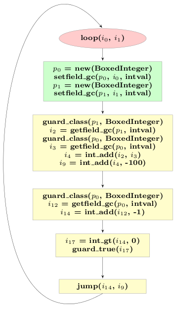
The final optimized trace of the example looks like this:
# arguments to the trace: p0, p1
guard_class(p1, BoxedInteger)
i2 = getfield_gc(p1, intval)
guard_class(p0, BoxedInteger)
i3 = getfield_gc(p0, intval)
i4 = int_add(i2, i3)
i9 = int_add(i4, -100)

guard_class(p0, BoxedInteger)
i12 = getfield_gc(p0, intval)
i14 = int_add(i12, -1)

i17 = int_gt(i14, 0)
guard_true(i17)
p15 = new(BoxedInteger)
setfield_gc(p15, i14, intval)
p10 = new(BoxedInteger)
setfield_gc(p10, i9, intval)
jump(p15, p10)
The optimized trace contains only two allocations, instead of the original five,
and only three guard_class operations, from the original seven.
Summary
In this blog post we described how simple escape analysis within the scope of
one loop works. This optimizations reduces the allocation of many intermediate
data structures that become garbage quickly in an interpreter. It also removes a
lot of the type dispatching overhead. In a later post, we will explain how this
optimization can be improved further.